Activation Functions

[From the last episode: We looked at the notion of sparsity and how it helps with the math.]

We saw before that there are three main elements in a CNNA type of artificial neural network specifically used for machine-vision applications.: the convolution, the pooling, and the activation function. Today we focus on activation functions.

I’ll start by saying that the uses of activation functions aren’t intuitively obvious, and, if you google around, you’ll find lots of deep mathematical discussion. That’s not the goal here. We’ll take a more general approach. It takes some serious math to understand all of this, and it’s very much an area for specialists – which I am not.

Linear vs. Non-linear

We can use some simple examples to illustrate the notion of linearity first. If you ask engineers why they use an activation function, a common high-level answer is to “add non-linearity.” Before we look at why that might be a good thing, let’s review what “linearity” means.

When something is “linear,” what we’re saying is that, when you graph it, it comes out as a straight line. Let’s look back at the function we defined a couple weeks ago: y(x) = x + 2. That graph was a straight line. So that function is linear. Functions with curvy graphs are not linear (we’ll look at some below).

Here’s the thing about linear functions: if you cascade them – say, do one linear function on an input, then do another linear one on the output of that one, and continue doing this, then you can replace that whole cascade with a single linear function. If we’re thinking about a deep neural networkA type of conceptual network organized in a manner inspired by our evolving understanding of how the brain works. that has lots of layers, that means that we could replace the whole networkA collection of items like computers, printers, phones, and other electronic items that are connected together by switches and routers. A network allows the connected devices to talk to each other electronically. The internet is an example of an extremely large network. Your home network, if you have one, is an example of a small local network. with a single layer – we’ve lost the value and nuance of a deep network.

Adding non-linearity to each layer now means that every layer has a very specific, and more complex, effect on the network.

Separating Values

Here’s another aspect to think about. Let’s say you’re trying to classify something as “dog” or “not dog.” You’ve got a bunch of inputs, and you’re trying to separate the bunches of inputs into those that are a dog and those that aren’t. If you plot the data, you’re really trying to find a separation from dog and not-dog inputs.

So the big question then becomes, what does that separation look like? Let’s say it looks like this, where we’ll assume that blue dots are samples that qualify as “dog” and red ones are “not dog”:

(Image credit: By Qwertyus – Own work, CC BY-SA 4.0)

We can see that the line separating “dog” from “not dog” is simply a straight line, and linear functions might be able to do this. This also shows that there are many ways to draw a line. The two lines shown both separate the red and blue dots – and there are infinitely many lines between them (roughly pivoting around the point where they cross) that could also work. This is an illustration of the thing we saw before: there’s no one right modelA simplified representation of something real. We can create models of things in our heads without even realizing we're doing it. Technology often involves models because they let us simplify what would otherwise be extremely detailed, complicated concepts by focusing only on essential elements..

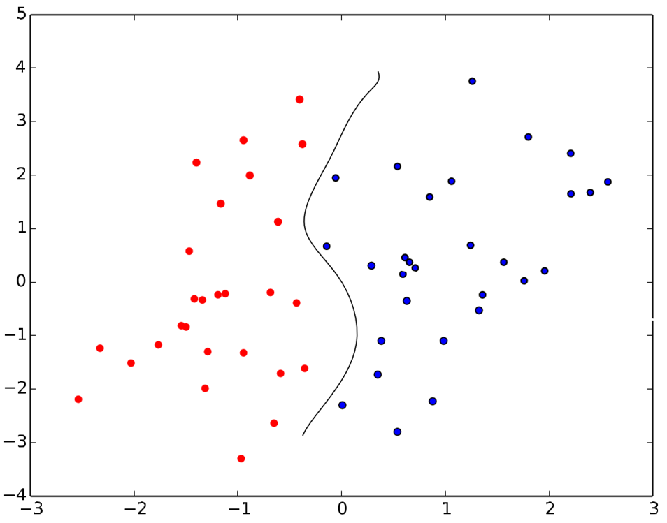
But what if the separation isn’t so clean – what if it’s curvy?

(Image credit: created by author based on prior image)

You can’t do this with a linear function; you need something that will bring some curves into the picture.

Training Benefits

The algorithmsA way of calculating something, typically as a step-by-step recipe. A familiar one to all of us is how we do long division on paper: that's an algorithm. Algorithms abound in the IoT. used for trainingWith machine learning, a model must be trained in order to perform its function (which is called inference). a network work backwards from an output. If the output is wrong, then they figure out the error and push that backwards through the network to adjust all the weights to where it would be right. At each layer, this includes pushing it back through the activation function. More nuanced learning is possible with this non-linearity, although the non-linear function has to have certain characteristics to be useful (we won’t dive into that).

Example Activation Functions

There are many, many possible functions that we could use – it’s even possible for a developer to create a custom function for a particular need. But there are a few more common functions, which we’ll describe here.

Just to be clear on how to interpret these if this isn’t obvious, what we’re looking at are graphs of these functions. What happens is that, for each data point you have, you look along the horizontal axis and find that point. You then multiply that point by the value of the function there.

ReLU (Rectified Linear Unit)

This is a really simple function. On the left side of the vertical line below (follow the blue line), the function always gives 0 (it runs along on top of the horizontal axis). Said another way, if you’re starting with a negative number, then you’re multiplying by something in the left-hand half of that graph (the blue part), which is always zero. That’s why this eliminates the negative numbers. On the right side, it gives whatever value you started with (or some proportional number).

This is easy to compute, making it popular for many networks. (The green line is another activation function called Softplus; we won’t discuss it).

(Image credit: CC0 on Wikipedia)

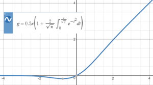
GeLU (Gaussian Error Linear Unit)

This is similar to ReLU except that it doesn’t completely zero out small negative numbers. (Yeah, that’s a funky-looking equation.

(Image credit: User named Esmailian on StackExchange)

Sigmoid

This generally describes a function that has a kind of “s” shape (“sigma” being the Greek letter for the S sound – so “sigmoid” means “in the form of a sigma” – even though the Greek form of sigma (∑) isn’t shaped like an S…). It gives a nice steepish slope near the horizontal axis’s zero point. The specific one shown below goes to zero on the very left, so large negative numbers will disappear. It goes to 1 on the far-right side, so it has no effect on those numbers (multiplying by 1 keeps the original number). In between, it almost looks like a straight line until the curvy parts start. So this function keeps big positive numbers while starting to reduce the effect of smaller positive and negative numbers until you get to the point where the negative numbers are (effectively) zeroed out.

(Image credit: By Qef (talk) – Created from scratch with gnuplot, Public Domain.)

Hyperbolic Tangent (tanh)

This is classically pronounced “tanch,” although these days you’ll often hear “tan-h”. It looks similar to a sigmoid; there are subtle mathematical distinctions between the two that we won’t get into. The following image shows several “hyperbolic trigonometry” functions; the dotted blue line is the one we’re interested in (and you can see that it’s similar to a sigmoid, although with 0 in the middle instead of 0.5 as shown in the sigmoid above).

(Image credit: By Fylwind at English Wikipedia – Own work, Public Domain.)